Testing Julia for speed (ii)

The next test for evaluating the performance of Julia uses the Bubblesort. 

Bubblesort is arguably one of the most infamous sorting algorithms, partially because it is simple, and partially because it is one of the worst performing sorting algorithms. It works by repeatedly passing through an array, comparing two items and swapping them if they are in the wrong order. A bubble sort has a worst case complexity of O(n²).

So how fast (or slow) is bubble sort? Here is the code in Julia.

function bubblesort(arr)
    n = length(arr)
 
    for i=1:n, j=1:n-i
        if (arr[j] > arr[j+1])
            arr[j], arr[j+1] = arr[j+1], arr[j]
        end
    end
end

arr=[]
for i=1:1000
  push!(arr,rand(1:10000))
end

bubblesort(arr)

Again, code in C, Fortran, and Python is similar, so I’m not going to reproduce it. Note the interesting use of the variable swapping syntax, and the ease with which a random array of numbers is created.

The timings for sorting 1000, and 100,000 random numbers is given below.

timingBubblesort

Again, C and Fortran have similar timings, with Julia approximately 5 times slower than either, for the large sort. The big eye opener is Python of course  which, having issues with loops, is over 16 times slower than Julia, and 89 times slower than C.

Note that all the code for these programs was written the same way, i.e. an efficient version of Bubblesort was not implemented. Both Julia and Python used their intrinsic syntax for swapping two numbers, versus the use of the swap() function in C and Fortran.


Testing Julia for speed (i)

The speed of a program shouldn’t really matter, I mean it is ultimately about how robust a program is, and how correct it’s output is. However in the age of big data, no-one really wants to wait an eternity  for a program to perform its tasks. Consider the task of developing an AI to beat a human at a board game such as chess – here the aim is to win, not necessarily to do it in any set time frame. However processing a large image or 3D data set ultimately requires some element of speed. In order to experiment with how fast Julia is we will use three algorithms: (i) Ackermann’s function, (ii) Bubblesort, and (iii) a simple mean-filter for image noise suppression applied to a large image. These will be used to compare Julia with C, Python, and Fortran.

Ackermann’s Function

Ackermann’s function was originally conceived in 1928 by Wilhelm Ackermann, and has been used extensively in the past for studies in computational efficiency, especially by B.A. Wichmann. Ackermann’s function is interesting from the point of view that it is a highly recursive function.  Ackermann’s function has the following recurrence relation:

ackermannFORM

This is expressed as a recursive function, which may seem simple, but the larger m and become, the more complex the recursion becomes. Due to the limitations Python has with recursion, we will use an iterative version of Ackermann, which relies on the use of stacks to implement recursion. Ackermann’s function is a classic function which serves no purpose other than evaluating computational performance.

The code for Python and Julia includes use of built-in functionality to implement a stack, whereas in C and Fortran the code for the stack is provided in the form of a library, and module respectively. Here is the Julia code to calculate the iterative version of Asckermann’s function.

function ackermannIterative(m,n)
    stack = []
    push!(stack, m)
    while (isempty(stack) == false)
        m = pop!(stack)
        if m == 0
            n = n + 1
        elseif n == 0
            push!(stack, m-1)
            n = 1
        else
            push!(stack, m-1)
            push!(stack, m)
            n = n - 1
        end
    end
    return n
end

print("Value m: ")
m = chomp(readline())
m = parse(Int, m)

print("Value n: ")
n = chomp(readline())
n = parse(Int, n)

@time result = ackermannIterative(m, n)
println("Ackermann : ", result)

To test the various languages, we will calculate Ackermann(4,1), which has a value of 65533.

timingAckermann

As is expected, C leads the pack, with Fortran trailing close by. This is not unexpected from two statically typed languages. Julia is approximately 4 times slower than C. Python is the outlier here, being more than 25 times slower than C, and 7 times slower than Julia. There is little that can be done to improve this code, as very little is calculated, it is merely involves some simple arithmetic, and calls to add and remove items from a stack.


Programming in Julia – the caveats

Not everything in Julia is great, like I’ve said before, there is no definitively perfect programming language. One of the caveats of the language is its size. Much of this size is also what makes it an exceptionally powerful language, so it is a bit of a catch-22. This discussion will concentrate on some of the more global issues.

Documentation

One of the biggest caveats I have encountered with Julia is the vagueness  of some of the documentation. The language itself is seemingly well documented, but does suffer from a lack of examples to illustrate how certain features work. Third party packages are another thing altogether – some seem to suffer from little or no documentation, and one is forced to searching on Stackoverflow for answers. A case in point is the module. Ideally, this is a means of encapsulating a series of related functions, so they can be easily ported. It took me over two hours to finally figure out exactly how they could work. The problem here is one of the language being in flux still, with changes to the syntax being made. Some of these issues may sort themselves out when a stable version is released.

Consistency

Programmers expect consistency. For the longest while I was running the scripts I wrote through the command line:

julia imageIO.jl

Now that worked fine, until I incorporated the use of a plotting function from the packages Gadfly (Julia has no built in visualization functions). It actually could not plot the histogram I wanted it to, so in the end I opened up Julia in interactive mode, and low and behold, it worked. Now Gadfly uses a browser window to display the graphics, which isn’t a problem. But running a script  means the following:

include("imageIO.jl")

Which doesn’t seem as intuitive as it could be. Used in any context the term include, suggests something more akin to how C uses it. Indeed, when I later created a module, it was “included” in another script using:

include("imageENH.jl")
using imageENH

This makes sense, but running a script should probably use something like “run”. Unless of course you are actually including a module in the main interpreter. There is some ambiguity here.

So, there seem to be two ways to write programs : the script, or the module (lets leave out packages for the moment). A script is a simple program which can contain any number of functions, and a “main” portion of the program at the bottom, essentially a script. A module encapsulates a series of functions, for the sake of reusability.

Deprecation

The problem with any new language is that it suffers from instability. Gone are the days when a language was designed in its entirety before it was implemented. Consider Algol as an example of this. The first version, known now as Algol 58 was designed by committee, and implemented in a limited manner. When the committee met in 1960 to consider its deficiencies, the language was redesigned to become Algol 60. It was not common for a language to be used as it was evolving. This is however common now, and Julia is a prime example, although it does lead to issues, one in particular is the idea of deprecation. This is not new of course, new versions of Fortran often deprecated older, obsolete syntax. A case in point is the Julia syntax for selecting only certain elements from an array. This was previous achieved using {a,b, …} which means a statement of the form b[{1,3}] would select the 1st and 3rd element of b. Now this has been deprecated, replaced by Any[a,b, …] or in the case of the example: b[Any[1,3]]. However if the range of indices is stored in an array, this syntax cannot be used, for example if d=[1,3], then choosing the 1st and 3rd elements of b would be performed as b[d]. Deprecation will obviously be less of an issue when the language stabilizes.

Error Messages

I have to say it. The error messages in Julia are less than optimal. Some have to do with runtime issues. For example, consider the following code snippet, which reads in an integer, creates an array of that size, assigns the value 1 to all elements, and attempts to print out element n+1:

print("A number: ")
n = chomp(readline())
n = parse(Int, n)
x = [1:n;]
x[1:end] = 1
println(x[n+1])

Here is the program running, with a BoundsError triggered:

JuliaBoundserror

In another piece of code, which uses = instead of == in a conditional,

print("A number: ")
n = chomp(readline())
n = parse(Int, n)

if n = 1
    println("Why?")
end

the following syntax error is issued:

JuliaSyntaxerror

While the information exists as to the type of error, and where it is, there is also a lot of trace information that may not be that useful to the novice programmer. In fact unlike other languages, error messages are not well localized. In fact they are often quite verbose.

IDIOSYNCRASIES

There are some idiosyncrasies which programmers have to look out for. When dealing with arrays, if an array is created:

arrayA = [1, 2, 3]

and then copied:

arrayB = arrayA

Then any changes made to arrayB will be reflected in arrayA – this is because arrayB is not a copy of arrayA, but merely references it. To make a copy requires the copy function:

arrayB = copy(arrayA)

INSTABILITY

Despite all the best intentions, there are still instabilities in the compiler. These manifest themselves in errors of the following form, which end up crashing the Julia session:

GC error (probable corruption) :
<?#0x10bd930c0::0x0>

signal (6): Abort trap: 6
__pthread_kill at /usr/lib/system/libsystem_kernel.dylib (unknown line)
Abort trap: 6

The same program run again works fine. I can only imagine there are memory issues.


Julia – Design in the small

Many people discussing Julia look to its claims relating to speed (vs. languages such as Python), and that is an important feature of a language built for crunching numbers.  Some people like to harp on the OO characteristics of a language, or it functional abilities, but it is the basic language structures, that make or break a language. It is easy to write programs in Julia. Part of this ease comes with a usable syntax, whilst other parts are attributable to the lack of low-level features, at least from the perspective of the novice user. Below we will discuss some of the more interesting features of Julia.

BASIC THINGS

One of the things I like, yet may make other people cringe, is the simplistic nature of some mathematical expressions. In math, an expression may be of the form x = 4a + b2. In C this would be written as:

x = 4 * a + b * b

But in Julia, it can be written as:

x = 4a + b^2

There are features of Julia that making writing expressions easier. For example, Julia is capable of directly evaluating a conditional expression such as 1<x<12, which in C would require an expression of the form: ((x>1) && (x<12)). Swapping the values stored in variables is also easy, using an expression of the form: a, b = b, a.

Some of the more interesting features of Julia include allowing variable names to use Unicode (UTF-8), so either the word “pi”, or π can be used. However it is also possible to use traditional numeric comparison operator, ≠ instead of !=, ≤ instead of <= etc. The only problem here might be the lack of practicality, i.e. keyboards, and might require some form of IDE to make usable.

Julia also does some interesting things with operators. Unlike C which overloads the division operator, Julia instead opts to use the function div(x,y), and replaces the % C uses for modulus with the function mod(x,y). It also introduces rem(x,y) to calculate the remainder. Types are consistent, meaning that Int8 implies an 8-bit integer, and Int64 a 64-bit integer. Unsigned integers are defined by prefixing with a U, e.g. UInt8. Floats are defined in a similar manner.

Control Structures

Control structures are similar to those found in other languages, however they do benefit from a usability standpoint. Julia essentially offers one conditional statement: if-elseif-else, there is no switch or equivalent. The if statement does not require the use of ( ) to delimit the conditional expression (but you can use parentheses if you like). There is also no ambiguity caused by the dangling else, such as in C, as all control structures are terminated with the end clause. Some people may see the addition of a control-structure terminator such as end adding verbosity to the language, but in reality it adds more clarity than anything else. Unlike C and Python, Julia also does not allow anything except a boolean evaluation in the conditional (so expressions like x = y are avoided).

There is no switch or similar statement in Julia, maybe because it offers no additional functionality over the if structure. The switch statement is one of the few which has to be very well designed, otherwise it can end up doing more harm than good. A switch statement would be a welcome addition to the language, but only if similar to that incorporated in Swift, rather than the ineffectual design of C.

From the perspective of loops, Julia provides only two: for and while. The while loop is similar to that found in other languages. The for loop, uses a much simpler syntax:

for i = 1:100
   ...
end

The for loop can also iterate over containers, using the keyword in.

for i in [1,1,2,3,5,8]
   ...
end

The keywords break and continue exhibit the same behavior as in C. As an interesting side, Julia allows multiple nested loops to be combined into a single outer loop, forming a “cartesian product of iterables”.

for i=1:100, j=1:100
   ...
end

Like its contemporaries (e.g. Swift), there is also no goto statement. Considering how ubiquitous exception handling is in Julia, I would argue that it is hardly needed. The exception handling is itself very much akin to that found in Ada. Here are a couple of examples:

BoundsError - array out of bounds
DomainError - sqrt(-1)

Julia also allows the programmer to define their own exceptions, offers warnings and informational messages that do not interrupt execution, and try/catch combinations to allow exceptions to be tested. This stops any of the problems confronted by novice programmers using languages such as C.

MODULARITY

Functions are easy to create.

Julia uses a single function format, there is no differentiation between functions that return values and those that don’t. Functions are identified using the keyword  function, as opposed to def from Python, or nothing like C/C++. There is no need to specify a return type, or use the keyword void. The value returned is the value of the last expression in the body of the function, or alternatively that associated with the traditional keyword return.  Functions can return multiple values in the guise of tuples, as well as mutable values. Julia also allows for an arbitrary number of arguments, and optional arguments (with a default value).

Unlike other languages such as C, Julia performs argument passing by “pass-by-sharing”, which means that values are not copied when they are passed to functions. Generally the arguments given to the function are not modified, except mutable values such as arrays (akin to pass-by-reference). This means there is no need for the novice programmer to worry about the difference between the different modes of passing parameters to a function. Unlike C, there is also no need to learn about pointers in order to use functions. Julia also provides libraries in the guise of a module.


Programming in Julia – First impressions

Programming languages have been evolving for over seventy years, but the last 40 years have focused heavily on languages based on the C lineage. The new languages we have seen born in the past 3-4 years have started to move away from the C-like syntax, and take on characteristics of languages past. Julia is one such language. One of Python’s strengths is fast prototyping, and an extensive cadre of libraries. However it suffers from being a slow dynamic language, and the requirement of having to re-write the code in a faster static language such as C or C++ when a “final” product is needed – something commonly known as the “two-language” problem.

The programming language Julia offers a solution to this: expedient building in a fast dynamic language.

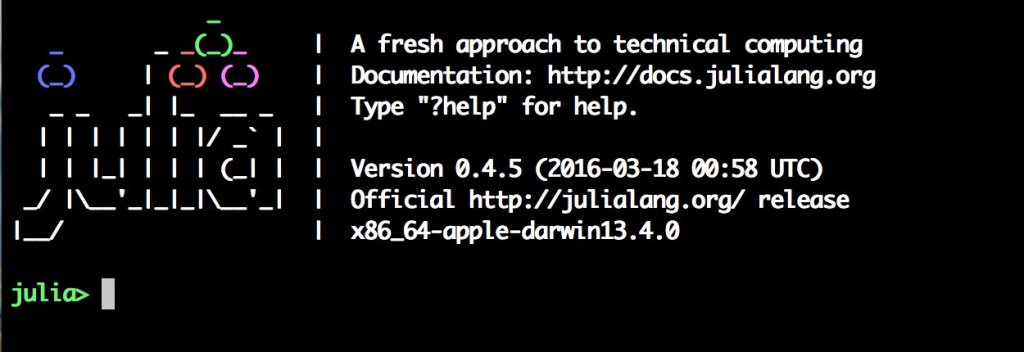
julia

Recently I spent a day trying to get a better handle on programming in Julia. There are a bunch of opinions on various blogs relating to experiences with Julia, mostly good. Julia has many good qualities, foremost of which is that it seems to be a very well designed language, with usability one of the guiding principles. It is primarily suppose to act as a scientific language, as a potential replacement for the likes of Python, and Fortran, and likely a low cost alternative to Matlab.

Julia, named after French mathematician Gaston Julia, the inventor of fractals, was publicly released in 2012. It was developed by Stefan Karpinski, Jeff Bezanson, Viral Shah, and Alan Edelman at MIT. The objective was to create a language by encompassing the positive attributes of numerous languages: Python (simplicity and dynamism), R (statistical processing), C (execution speed), Perl (string processing), and Matlab (linear algebra). Julia is by no means a small language. It has a whole lot of functionality, mostly in the form of data structures, such as arrays and stacks, and their associated functionality. In that respect it is less of a traditional language with a low form factor, such as C. But it makes up for it in the extensive functionality.

I use Julia mainly for image processing, so the gripes I have with: C (use of dynamic arrays for large images, and lack of libraries); Python (syntax, and slowness), and MATLAB ($$$, proprietary nature), just don’t exist with Julia. It is seemingly fast, and doesn’t have a coronary when I give it a large array to process in a nested loop. It allows me to specify types if I need to, but doesn’t make me have to figure out which is the best types for the data. In some forthcoming posts, I will outline some of the features of Julia as they relate to common programming constructs, and look at a few language comparisons with respect to performance.

A lesson in life

It’s been over 25 years since I finished my undergrad B.Sc. I went to university because my parents wanted me to go. I would have been just as happy becoming a carpenter, building things. I chose a university in the middle of nowhere in Australia, and never visited it before the day I started there. I was forbidden to become an architect, which is what I would have likely enjoyed doing, because my father was a draftsman. He disliked architects, to put it mildly. Initially I got accepted at the university to do agriculture (which *nobody* had an issue with, when you think about it is kind-of bizarre). I guess I never really put a lot of effort into choosing a university course because my heart really wasn’t in it. I changed to science before I had even chosen classes. In my first year I took biomath (i.e. math for biologists), chemistry (which I loathed), biology, and computer science. Biology seemed like a good choice, and some of the zoological stuff seemed kinda interesting (i.e. insects), but the botany part was dead boring, and overall it involved far too much rote learning, which I’m hopeless at. I had bad experiences with chemistry in high school, and never thought I would have to see it again – I was wrong, and ended up taking it for a second time in 2nd year. Math, well it was okay, half statistics, and next to no calculus.

The odd-ball course was computer science – I had never written a program in my life. Sure, we had an Apple IIe at home, but all I did on that was write BASIC “programs” with PRINT statements to print out essays, because I didn’t have a word processor. So I took the introductory course and learnt Pascal. Turns out programming was one of the few things that I was adept at, probably because it required you to build things. There were aspects that didn’t really interest me – theoretical stuff, hardware, assembler. But programming was fun. In the late 1980s programming was Pascal, C, Cobol, Fortran, and maybe Ada. And one of the shell languages. I took a “software engineering” course in my last year, but dropped it because I really felt it was lots of “mumbo-jumbo”. This was an early rendition of software engineering in a beginning of the era of OO. In the late 80s there was very little in the way of “software” type courses – everything was focused on programming. There were no group projects, or even larger-scale projects – and no design documents. Ironically I went on to get more degrees in computer science – because life lead me in that direction. I still enjoy programming immensely, learning new languages, and “building” software. As an undergrad I ended up taking 10 CS courses (that’s all there was).

First Year
Introduction to Programming I (Pascal)
Introduction to Programming II (Pascal)

Second Year
Unix and C
Computer Architecture & Assembler
Cobol & Introduction to Databases
Data Structures

Third Year
Compilers and Grammars
Comparative Study of Languages
Advanced Databases
An Introduction to Parallel Processing

In addition I took a numerical math and a computational math course involving Fortran.

My honours thesis (a separate 1-year degree in the British system) was on object-oriented problem solving in C++. By the end of my undergraduate degree I could program in Pascal, C, C++, Fortran, Ada, Cobol, and a bunch of shell scripting. I dabbled in some Prolog and Lisp, but never really found a passion for them as languages. Most of the work as undergrads was done on Unix systems, on the command-line. Few relevant compilers were available for DOS/Windows – these machines were still only bootable via a 5-1/4” floppy disk.

I learnt more in my first job, working in the Cartographic Services Unit of the Australian Geological Survey Organisation. They made maps, on huge Unix-based CAD machines, and PCs. GIS was just coming into the fray. Some of the other equipment was *old*. PDP-11 machines that had to boot off two magnetic tapes, and had monster 20MB disks attached. Huge drum scanners and plotters, that would produce maps. Networking, but no internet as we know it today. Here was where the practical stuff was learnt – rebuilding PC’s getting networks to work, playing around with configuration files, and drivers for idiosyncratic pieces of add-on boards.

25 years later, machines are still machines, and programs are still being written in languages such as C, Fortran, C++ and Cobol. Machines are faster and smaller, programming languages are more complex, software is ballooning in size, and design has become far too complicated. But at the end of the day we are still writing programs to solve problems.