2D array subscripts in Python

How the subscripts of multi-dimensional arrays is coded in Python really does matter. The element (i,j) of a two-dimensional array can either be written as:

X[i][j]
X[i, j]

Which is better? We took the naive box filter algorithm from the previous post, using each of these subscripting methods. The result:

X[i][j] - 84.19 sec
X[i, j] - 72.15 sec

So X[i,j] = X[i][j], but X[i][j] is more inefficient because a new temporary array has to be created after the first index that is subsequently indexed by j.

Image processing in Python – code efficiency

One thing you will quickly come to terms with in Python is that if you code things the wrong way – they will run slowly. To illustrate this, let’s consider a simple box filter – it basically assigned each pixel the average of all the pixels in a neighbouring region. For example, a 5 x 5 box filter centred on pixel I[i,j] will assign to pixel [i,j] in the processed image, the average of the region I[i-2:i+2, j-2:j+2]. It has the effect of smoothing the image and suppressing noise artifacts – the larger the neighbourhood, the more profound the smoothing effect. We’ll test four ways of applying the box filter in Python. For the experiment, the following image (415 × 751)  is processed.

noise_1

The result is a smoothed image.

noise_Box3

Here’s a close-up of before (left) and after (right) applying the box filter.

noise_boxEG

Method 1
This is the most naive approach to coding the solution in Python, yet in languages like C, this is usually the only approach due to the lack of ability to use sub-arrays. It does work, but is extremely slow – it takes 78 seconds to process this relatively small image.

def BoxFilter1(im, r=2):

    imS = numpy.zeros(im.shape,dtype=numpy.float)
    rN = (r*2+1)**2.0

    nr, nc = im.shape
    for i in xrange(r, nr-r):
        for j in xrange(r, nc-r):
            for k in xrange(-r, r+1):
                for l in xrange(-r, r+1):
                    imS[i, j] += im[i-k, j-l] / rN
    return imS

Method 2
In the second approach, the code processes the 5×5 neighbourhood without explicitly looping over each pixel in the image. This is achieved by means of vectorization. It relies on the use of numpy – the normalization and addition of the elements of the image are vectorized, releasing the outer two loops from the Method 1 which cycled through each element in the array. This leaves only two small loops: e.g., in the first cycle through the loops, the “neighbourhood” element at position [-2,-2] associated with each pixel in the image is normalized (divided by 25) and added to the pixel in the output image. Next cycle around the loop, neighbourhood element [-2,-1] is processed, etc. until all 25 elements have been processed. The algorithms speed? – 0.132 seconds – 590 times more efficient.

def BoxFilter2(im, r=2):
    rN = (r*2+1)**2.0
    nr, nc = im.shape
    imS = numpy.zeros((nr-2*r,nc-2*r),dtype=numpy.float)
    for k in xrange(-r, r+1):
        for l in xrange(-r, r+1):
            imS += im[r+k:nr-r+k, r+l:nc-r+l] / rN
    return imS

Method 3
In the third approach rather than vectorize the image, the numpy function sum is used to sum the pixel values in the neighbourhood for each pixel in the image. The algorithms speed? – 7.31 seconds – only 10 times more efficient.

def BoxFilter3(im, r=2):
    rN = (r*2+1)**2.0
    nr, nc = im.shape
    imS = numpy.zeros(im.shape,dtype=numpy.float)
    for i in xrange(r, nr-r):
        for j in xrange(r, nc-r):
            imS[i, j] = numpy.sum(im[i-r:i+r+1, j-r:j+r+1]) / rN
    return imS

Method 4
In the final approach the convolve function is used from the scipy.ndimage package (with a 5 x 5 box filter). The algorithms speed? – 0.11 seconds – slightly more efficient than Method 2.

def BoxFilter4(im):
    k1 = numpy.array([[1, 1, 1, 1, 1],
                      [1, 1, 1, 1, 1],
                      [1, 1, 1, 1, 1],
                      [1, 1, 1, 1, 1],
                      [1, 1, 1, 1, 1]])/25.
    imS = nd.convolve(im, k1, mode='constant', cval=0.0)
    return imS

Every different coding approach (and there are probably more) has a different outcome – yet they all prescribe to the same algorithm. How fast your algorithm runs will be largely dependent on the coding methodology best suited to the language you are using.

Does haze suppression really work?

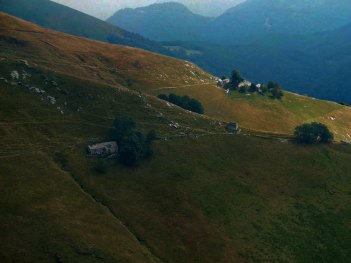
There are a lot of algorithms -especially in areas like image processing that *seem* like they work really well. Sometimes I wonder if this is because they have been tested on images where the results are really quite impressive. Take for example the task of haze suppression in photographs. I have run a couple of algorithms on some images with real haze in them and to be honest the results are quite good. The photographs were taken on Monte Generoso in the Swiss Canton of Ticino.  Here’s the first result. Clearly the background haze in the valley has been suppressed, but not totally removed. The colours are more saturated and vibrant – but do they now lack natural colour?

haze3s haze3_suppEGs

This algorithm runs reasonably quickly on the original at 3000 x 4000 pixels – 252 seconds – that may seem like a long time, but these algorithms are intrinsically complex. Too complex for a mobile device. Let’s try algorithm number two. Here’s the result. Is it better? The colours certainly don’t seem as over-saturated, and it appears as though more haze has been removed.

haze_30per haze30_suppEG

The problem here is speed. I down-sampled the image here to 600×800, and the running time was 112 seconds. For a 900×1200, 364 seconds. You can see where this is going. The larger the image, the more it struggles to get the processing done. Both algorithms were written in Matlab. As a second example, consider this image, again from the same area – haze was particularly bad that day.

haze1_30

The first image shows the result of processing with Alg.1, the second with Alg.2. The first algorithm seems to have left some hazy artifacts near the barn and rocks on the hillside. The second algorithm seems to have suppressed the haze better, and although being a little darker retains more of the image detail. The caveat – 433 seconds on a 900 x 1200 image.

haze1_alg2s haze1_30_alg1

To make these into a competent app, or even a “filter” on a camera would require some incredulous increase in efficiency. Algorithm 2, which produced the better visual results would take over 100 minutes to process the original 3000 x 4000 pixel photograph.

Beauty of course is truly in the eye of the beholder.

In Python loops can be lethal

I like Python, it’s a great language. What don’t I like? It’s slow. The thing is, you can’t just convert code from C to Python and hope it will run at the same speed. It won’t. This message came across loud and clear when I started doing image processing using Python. Algorithms that ran efficiently in C and Matlab became bogged down in Python. Maybe the core reason is that Python code executes slower because it is interpreted, rather than being compiled into native machine code. Built-in operations that improve efficiency in Python are typically pre-optimized – that’s why it’s good to use them. One of the biggest problems it seems is loops.

Write a small program using loops and this isn’t at all obvious. Write code to process a 3000 x 4000 pixel image, and you’ll see why. Consider the following Python code which converts an image from RGB to another colour space YIQ. Note that img is a numpy array, but the calculations are done using primitive operations.

for i in range(0,img.shape[0]):
    for j in range(0,img.shape[1]):
        imgY[i,j,0] = 0.299 * img[i,j,0] + 0.587 * img[i,j,1] + 0.114 * img[i,j,2]
        imgI[i,j,1] = 0.596 * img[i,j,0] - 0.275 * img[i,j,1] - 0.321 * img[i,j,2]
        imgQ[i,j,2] = 0.212 * img[i,j,0] - 0.523 * img[i,j,1] + 0.311 * img[i,j,2]

This code runs through each pixel individually, converting it from RGB (img), to the individual components of YIQ (imgY, imvI, imgQ). And it is slow. How slow? For a RGB image that is 3000 x 4000 pixels in size – 1004 seconds.

Now consider a better way of writing this piece of code, written using numpy operations.  Numpy is based on the “ndarray”, for n-dimensional array, data structure. These arrays are strided views on memory – where strides are  the number of bytes to skip in memory to proceed to the next element. Numpy also uses vectorization, where an operation is applied to all elements in the array. Vectorized operations in NumPy are implemented in C.

r, g, b = img[:,:,0], img[:,:,1], img[:,:,2]
imgY = 0.299 * r + 0.587 * g + 0.114 * b
imgI = 0.596 * r - 0.275 * g - 0.321 * b
imgQ = 0.212 * r - 0.523 * g + 0.311 * b

This piece of code works by performing the operations as a complete block, avoiding the use of loops altogether. The operations are automatically mapped to each element. How long does this take? 1 second.

Which goes to show that understanding how a programming language works goes a long way to writing efficient programs. Another image filtering example in Python will follow soon.

NB: An excellent paper on the Numpy data structure can be found here.

Why IDEs lead you to the dark side.

When I learnt to program it was on an archaic mainframe system in Pascal. A “when I was a boy we had to boot up the VAX using tape spools” kind-of story. But in reality, in the five years I spent as an undergrad command-line programming was all we ever did. There were no GUIs, and certainly no IDEs – the ubiquitous “Integrated Development Environment”. Now many want to program using an IDE. Sure it colours the code nicely, and makes things ever so easy – but what has been lost along the way? Mostly the art of tinkering with your code.

With command-line programming you delve into the lower level of the machine itself. To learn to program in C on a Unix system you had to learn about the shell, and the commands that help investigate and manipulate the system. You learnt that it you delete a file using rm then it wasn’t coming back. There was no unrm. It was a lesson learnt very quickly. If your program went haywire you could find the process and kill it. Sure you had to learn to use vi to edit your program – but it wasn’t the worst thing in the world. A lot of what we learnt was learnt by playing with the system. Runtime error messages  of the form “segmentation fault” were deciphered by trial-and-error – now where is that memory problem?

Novice programmers should start by learning to code using the command line. They will no doubt migrate to IDEs at some point, but they need to learn the how the system levels works – awk, grep, sed, cron – and the power of shell scripting languages. Yes, the command line can be scary. Get over it. Cobol is much scarier.